Numerical integrals and error

What about when we cannot integrate a function analytically? In other words, when there is no (obvious) closed-form solution. In these cases, we can use numerical methods to solve the problem.

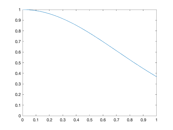
Let’s use this problem:

\begin{align} \frac{dy}{dx} &= e^{-x^2} \\ y(x) &= \int e^{-x^2} dx + C \end{align}

(You may recognize this as leading to the error function, \(\text{erf}\): \(\frac{1}{2} \sqrt{\pi} \text{erf}(x) + C\), so the exact solution to the integral over the range \([0,1]\) is 0.7468.)

x = linspace(0, 1);
f = @(x) exp(-x.^2);
plot(x, f(x))
axis([0 1 0 1])

Numerical integration: Trapezoidal rule

In such cases, we can find the integral by using the trapezoidal rule, which finds the area under the curve by creating trapezoids and summing their areas:

\begin{equation} \text{area under curve} = \sum \left( \frac{f(x_{i+1}) + f(x_i)}{2} \right) \Delta x \end{equation}

Let’s see what this looks like with four trapezoids (\(\Delta x = 0.25\)):

hold off
x = linspace(0, 1);
plot(x, f(x)); hold on
axis([0 1 0 1])

x = 0 : 0.25 : 1;

% plot the trapezoids
for i = 1 : length(x)-1
    xline = [x(i), x(i)];
    yline = [0, f(x(i))];
    line(xline, yline, 'Color','red','LineStyle','--')
    xline = [x(i+1), x(i+1)];
    yline = [0, f(x(i+1))];
    line(xline, yline, 'Color','red','LineStyle','--')
    xline = [x(i), x(i+1)];
    yline = [f(x(i)), f(x(i+1))];
    line(xline, yline, 'Color','red','LineStyle','--')
end
hold off

Now, let’s integrate using the trapezoid formula given above:

dx = 0.1;
x = 0.0 : dx : 1.0;

area = 0.0;
for i = 1 : length(x)-1
    area = area + (dx/2)*(f(x(i)) + f(x(i+1)));
end

fprintf('Numerical integral: %f\n', area)
exact = 0.5*sqrt(pi)*erf(1);
fprintf('Exact integral: %f\n', exact)
fprintf('Error: %f %%\n', 100.*abs(exact-area)/exact)

Numerical integral: 0.746211
Exact integral: 0.746824
Error: 0.082126 %

We can see that using the trapezoidal rule, a numerical integration method, with an internal size of \(\Delta x = 0.1\) leads to an approximation of the exact integral with an error of 0.08%.

You can make the trapezoidal rule more accurate by:

• using more segments (that is, a smaller value of \(\Delta x\), or
• using higher-order polynomials (such as with Simpson’s rules) over the simpler trapezoids.

First, how does reducing the segment size (step size) by a factor of 10 affect the error?

dx = 0.01;
x = 0.0 : dx : 1.0;

area = 0.0;
for i = 1 : length(x)-1
    area = area + (dx/2)*(f(x(i)) + f(x(i+1)));
end

fprintf('Numerical integral: %f\n', area)
exact = 0.5*sqrt(pi)*erf(1);
fprintf('Exact integral: %f\n', exact)
fprintf('Error: %f %%\n', 100.*abs(exact-area)/exact)

Numerical integral: 0.746818
Exact integral: 0.746824
Error: 0.000821 %

So, reducing our step size by a factor of 10 (using 100 segments instead of 10) reduced our error by a factor of 100!

Numerical integration: Simpson’s rule

We can increase the accuracy of our numerical integration approach by using a more sophisticated interpolation scheme with each segment. In other words, instead of using a straight line, we can use a polynomial. Simpson’s rule, also known as Simpson’s 1/3 rule, refers to using a quadratic polynomial to approximate the line in each segment.

Simpson’s rule defines the definite integral for our function \(f(x)\) from point \(a\) to point \(b\) as

\begin{equation} \int_a^b f(x) \approx \frac{1}{6} \Delta x \left( f(a) + 4 f \left(\frac{a+b}{2}\right) + f(b) \right) \end{equation}

where \(\Delta x = b - a\).

That equation comes from interpolating between points \(a\) and \(b\) with a third-degree polynomial, then integrating by parts.

hold off
x = linspace(0, 1);
plot(x, f(x)); hold on
axis([-0.1 1.1 0.2 1.1])

plot([0 1], [f(0) f(1)], 'Color','black','LineStyle',':');

% quadratic polynomial
a = 0; b = 1; m = (b-a)/2;
p = @(z) (f(a).*(z-m).*(z-b)/((a-m)*(a-b))+f(m).*(z-a).*(z-b)/((m-a)*(m-b))+f(b).*(z-a).*(z-m)/((b-a)*(b-m)));
plot(x, p(x), 'Color','red','LineStyle','--');

xp = [0 0.5 1];
yp = [f(0) f(m) f(1)];
plot(xp, yp, 'ok')
hold off
legend('exact', 'trapezoid fit', 'polynomial fit', 'points used')

We can see that the polynomial fit, used by Simpson’s rule, does a better job of of approximating the exact function, and as a result Simpson’s rule will be more accurate than the trapezoidal rule.

Next let’s apply Simpson’s rule to perform the same integration as above:

dx = 0.1;
x = 0.0 : dx : 1.0;

area = 0.0;
for i = 1 : length(x)-1
    area = area + (dx/6.)*(f(x(i)) + 4*f((x(i)+x(i+1))/2.) + f(x(i+1)));
end

fprintf('Simpson rule integral: %f\n', area)
exact = 0.5*sqrt(pi)*erf(1);
fprintf('Exact integral: %f\n', exact)
fprintf('Error: %f %%\n', 100.*abs(exact-area)/exact)

Simpson rule integral: 0.746824
Exact integral: 0.746824
Error: 0.000007 %

Simpson’s rule is about three orders of magnitude (~1000x) more accurate than the trapezoidal rule.

In this case, using a more-accurate method allows us to significantly reduce the error while still using the same number of segments/steps.

Error

Applying the trapezoidal rule and Simpson’s rule introduces the concept of error in numerical solutions.

In our work so far, we have come across two obvious kinds of error, that we’ll come back to later:

• local truncation error, which represents how “wrong” each interval/step is compared with the exact solution; and
• global truncation error, which is the sum of the truncation errors over the entire method.

In any numerical solution, there are five main sources of error:

1. Error in input data: this comes from measurements, and can be systematic (for example, due to uncertainty in measurement devices) or random.
2. Rounding errors: loss of significant digits. This comes from the fact that computers cannot represent real numbers exactly, and instead use a floating-point representation.
3. Truncation error: due to an infinite process being broken off. For example, an infinite series or sum ending after a finite number of terms, or discretization error by using a finite step size to approximate a continuous function.
4. Error due to simplifications in a mathematical model: “All models are wrong, but some are useful” (George E.P. Box) All models make some idealizations, or simplifying assumptions, which introduce some error with respect to reality. For example, we may assume gases are continuous, that a spring has zero mass, or that a process is frictionless.
5. Human error and machine error: there are many potential sources of error in any code. These can come from typos, human programming errors, errors in input data, or (more rarely) a pure machine error. Even textbooks, tables, and formulas may have errors.

Absolute and relative error

We can also differentiate between absolute and relative error in a quantity. If \(y\) is an exact value and \(\tilde{y}\) is an approximation to that value, then we have

• absolute error: \(\Delta y = | \tilde{y} - y |\)
• relative error: \(\frac{\Delta y}{y} = \left| \frac{\tilde{y} - y}{y} \right|\)

If \(y\) is a vector, then we can define error using the maximum of the elements:

\begin{equation} \max_i \frac{ |y_i - \tilde{y}_{i} |}{|y_i|} \end{equation}